Machine Learning and BGP Anomaly Detection

Border Gateway Protocol

The Border Gateway Protocol (BGP) helps to coordinate and maintain connectivity among Autonomous Systems (AS), providing a reliable and stable mechanism for service providers, CDNs, and enterprises to exchange routing information.

However, abnormal events such as link failures, misconfigurations, worm attacks, and prefix hijacks can affect BGP performance, destroying the stability and accessibility of the global internet. Therefore, detecting any abnormal BGP events is extremely important.

In April 2017, the Swiss operator SwissIX initiated a prefix hijacking attack, affecting the accessibility of 3431 and 576 AS prefixes globally, including Apple, Amazon, and Google. This incident, among many, is forcing service providers like Cloudflare to take additional measures.

If BGP anomalies can be detected with effective countermeasures, their impact on global Internet accessibility and stability can be significantly reduced. Fortunately, there are many machine learning (ML) techniques for BGP anomaly detection. For example, there are “machine learning methods that have improved BGP anomaly detection using volume and path features of BPGs update messages, which are often noisy and bursty.” In this post, we will explore the different types of BGP anomalies and how ML tools help detect and prevent them.

Types of BGP Anomalies

Based on the consequences of events, BGP anomalies can be classified into two categories:

Data flow hijacking anomalies: These anomalies can result in the redirection of the victim network data flow and/or a traffic black hole. This hole destroys the accessibility of the victim network.
BGP update messages explosion anomalies: As a result of these anomalies, a large number of BGP update messages are generated in a very short time. It leads to destabilized stability of the global Internet.

Machine Learning Techniques For BGP Anomalies Detection

Machine learning models are the most common and effective approaches for classifying and identifying BGP anomalies. Some of these techniques are discussed below.

Support Vector Machine (SVM)

SVM is a supervised learning model designed for classification and regression. It uses labeled training samples to learn a classification hyperplane by maximizing the minimum distance between data points that relate to various different classes.

There are two SVM models:

Hard-margin: These SVMs require each data point to be correctly classified.
Soft-margin: These SVMs allow misclassification of some data points to be misclassified.

To acquire hyperplane, users have to solve a loss function (1) with constraints (2):

C × Σ N n=1ζn + 1 2 ||w|| (1)

tny(xn) > 1 − ζn, n = 1, …, N, (2)

Here, parameter C > 0 controls the trade-off between the penalty term and margin.

N: number of data points
Ζn: slack variable
Tn: target value
y(xn): the training model
Xn: data points.

The following figure shows the illustration of the soft margin:

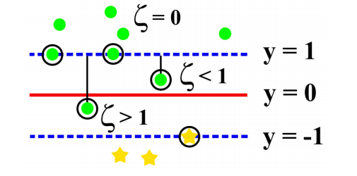
The solid line in this figure represents the decision boundary, and dashed lines represent the margins. Data points with circles indicate support vectors.

The perpendicular distance between the closest support vectors and the decision boundary represents the maximum margin. Data points ζ = 0 are correctly classified and are either on its correct side or on the margin. Data points 0 ≤ ζ < 1 lie inside the margin and on the correct side of the decision boundary. Data points for which ζ > 1 lie on the wrong side of the decision boundary and are misclassified.

The SVM computes a nonlinear separable function using a kernel function. Then, it converts the feature space into a linear space. The Radial Basis Function is recommended because it outperforms other types of SVM kernels and creates a large function space:

K(u, v) = exp(−λ||u − v||2 )

Here, v and u are dataset matrices. Constant λ affects the count of support vectors. Parameters λ and C are chosen using 10-fold cross-validation when generating the SVM models.

Long Short-Term Memory (LSTM) Neural Network

The LSTM neural network approach uses a special form of Recurrent Neural Networks (RNNs). In comparison to the RNN model, conventional RNNs store inputs to predict the outputs. But, their performance degrades when discrete-time lags take place between the previous inputs and the present targets. On the other hand, LSTM connects time intervals to create a continuous memory. It is designed to overcome any potential vanishing gradient problems.

Implementation of the LSTM consists of an LSTM layer, an input layer, and an output layer. The input layer has 37 nodes that serve as inputs to the LSTM layer. Each of these 37 nodes corresponds to one feature. Next, the output layer features one node connected to the LSTM layer’s output. The output is labeled by -1 (regular) or 1 (anomaly).

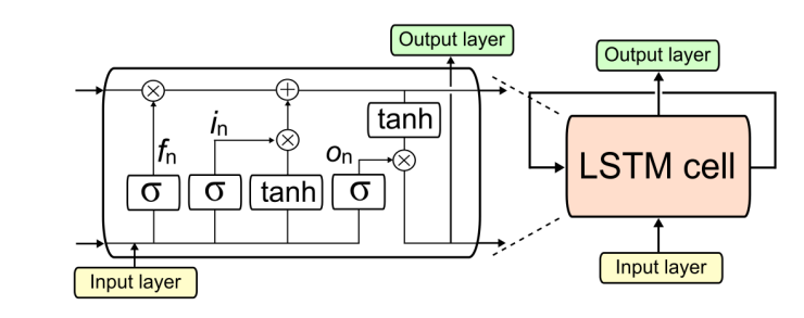
When it comes to the LSTM layer, it features one LSTM cell that is termed as a “memory block”. It consists of a forget gate fn, input gate in, and an output gate on.

The forget gate uses the cell state to determine useless memories and discards it. The input gate controls all the information updated in the LSTM cell. The output gate serves as a filter to the output.

The following figure shows an LSTM module. Here, tanh and σ denote the network output and the logistic sigmoid functions, respectively.

BGP Anomaly Prediction Based On The Ensemble Learning

Ensemble learning is a machine learning model that employs several different classifiers to reliably identify BGP network anomalies. By combining multiple classifiers, ensemble methods improve performance measures.

Here, we will use boosting, bagging, and random forest ensemble models trained on network anomaly datasets for classification improvement.

Bagging

Begging is one basic ensemble method that is based on the creation of different datasets. These datasets are based on the original training dataset, Begging combines these datasets into one model based on the majority vote rule.

Random data sampling with replacement from the original dataset generates new datasets. Every training dataset is independent, and some particular instances from the original dataset could occur multiple times in the new dataset, while some could be omitted.

The training datasets could be a little different when paired with weak classifiers that change their classification performance upon a small change in the training dataset.

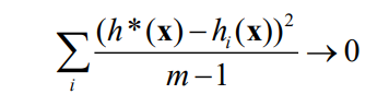
With the bagging method, the following variance expression can be reduced if m (the number of models) is high:

Boosting

AdaBoost or Adaptive Boosting is the first effective boosting algorithm used for binary classification. The generated model allows weights to be applied to the training dataset.

The weights are decreased or increased according to the previous models. Also, a majority vote is applied for accurate models to have a greater influence in the voting.

Therefore, a classifier with accuracy under 0.5 has a negative weight factor, and the classifier with accuracy more than 0.5 receives positive weighting factors. AdaBoost adds models successively until it generates a hypothesis that classifies the training dataset or the predetermined maximum number of models is reached.

Unlike with the most learning algorithms in which the error between the testing and training models increases as the complexity of the model rises, with AdaBoost, an increase of the number of iterations results in equalizing or even decreasing the difference between the model training and testing errors. That is because the margin on a training dataset is higher with smaller errors.

The following equation represents the final classifier made of the K weak classifiers:

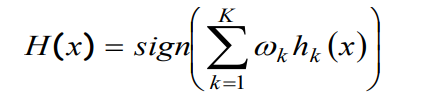
Hk: hypothesis of the weak classifier

ωk: weighting factor

Here is the equation to calculate the classifier error:

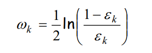
εk: Number of misclassified instances divided by total instances in the training dataset. εk k → 0 means the weighting factor increases exponentially, for 0.5 k → it is zero, and for 1 k → the weighting factor decreases exponentially.

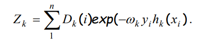
For calculated k and in accordance with equation (4), we determine the weights for the i-th instance from the training dataset:

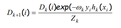
where Dk (i) is a vector of weighting factors to be used during the training of the k-th classifier. Weight factors represent that the i-th instance would be selected as the training dataset.

hk and yi could have two possible values since it is a binary classification. Hence their product could be -1 or 1. If the actual and predicted value is the same, their product is positive, and if they differ, the product is negative

The boosting method with increased iterations overfits much slower when compared to a model that is based on other methods. Soft margins enrich the boosting method, and it is widely used in RegBoost, Linear Programming Boost, Ada-BoostReg, and Quadratic Programming Boost. Soft margins and slack variable implementation are also applied in Support Vector Machines.

Random Forest

The Random Forest algorithm uses the bagging method AdaBoost. The use of a decision tree speeds up, generating a classification model. The model has limited complexity and limited accuracy of the training set.

The Random Forest Method improves accuracy with the increasing complexity of the trained classification model. This model follows the principle that in a randomly chosen space that is a subset of the original space of features, it produces different decision trees, such as T1, T2, .., TN.

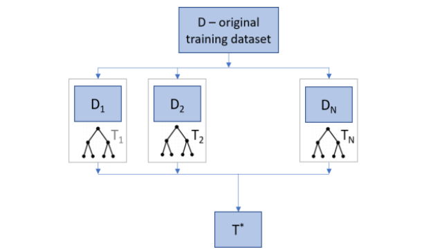
The Random Forest ensemble method uses k randomly selected features to divide the feature space. For the best results, the bagging method can be combined with a randomly selected features subset.

Combining these generated decision trees increases classification accuracy. It also leads to independence between the trees that make up the random forest. You can implement this method in parallel. It also effectively deals with input features and the data in which distributions are unknown.

Experiment and Analysis

Datasets imbalance makes it inappropriate to measure the model’s classification effect only by the classification accuracy. That’s why it makes sense to use the F1-Score and classification accuracy to evaluate the model’s performance.

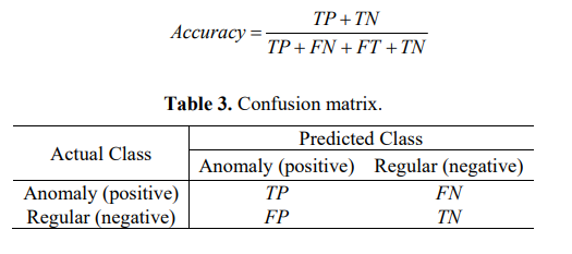
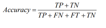
Classification Accuracy: It is calculated according to the classification confusion matrix, as shown below:

For binary classification, it is divided into four cases: FP, FN, TP, and TN.

TP: The sample and prediction result is positive
FN: Positive sample, and negative false prediction
FP: Negative
sample and positive prediction
TN: The sample is negative, and the prediction is negative.

The classification accuracy can be defined as:

F1-Score: It refers to the weighted harmonic value on an average of recall and precision. The precision is used for predictions that indicate the number of samples with positive predictions tend to be true positive samples. On the other hand, recall is for the original sample that indicates the number of positive examples in the sample is predicted appropriately.

Precision, recall, and F-Score are defined as follows:

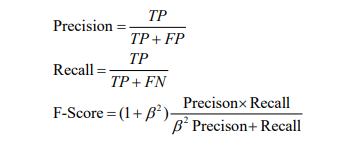
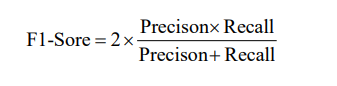
β > 0 refers to the importance of recall and precision. Let’s assume that β =1 which means precision and recall are equal in value. Accordingly, the F1-Score formula is:

Fisher-Markov Selector Feature Selection algorithm

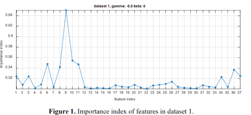
You get the importance index θ for each feature from the training dataset. This dataset is provided by Fisher-Markov Selector feature selection algorithm.

The following three figures show this respectively: Dataset 1

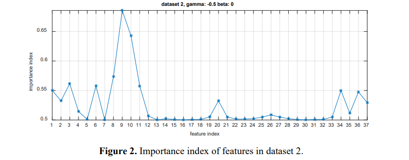
Dataset 2

Dataset 3

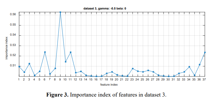
The following table shows the feature index and the corresponding importance index θ.

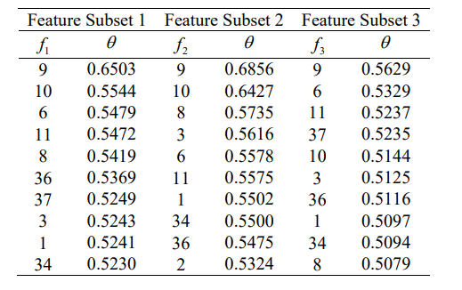
Top 10 features are chosen from dataset 1 and 3, and all are the same. It is because the Fisher Markov Selector feature selection algorithm is properly adapted.

Summary

Although much of the research on machine learning and networking is being done in academia, commercial enterprises are starting to craft their own methods that use ML. Experimental results depict that the SVM and ML-powered neural networks are valid methods.

Sometime in the future, machine learning will become a dominant part of not only detecting and/or preventing BGP problems, but also improve latency and packet loss.

Resources:

L. Jean Camp: Using ML to Block BGP Hijacking
Packet Routing in Dynamically Changing Networks
A comprehensive survey on machine learning for networking
MIT: Profiling BGP Serial Hijackers
A Framework for BGP Abnormal Events Detection
Comparing Machine Learning Algorithms for BGP Anomaly Detection using Graph Features
Application of machine learning in BGP anomaly detection
A Machine Learning Approach to Routing